
Abstract
Now that ever more sophisticated devices for quantum computing are being developed, we require ever more sophisticated benchmarks. This includes a need to determine how well these devices support the techniques required for quantum error correction. In this paper we introduce the topological_codes module of Qiskit-Ignis, which is designed to provide the tools necessary to perform such tests. Specifically, we use the RepetitionCode and GraphDecoder classes to run tests based on the repetition code and process the results. As an example, data from a 43 qubit code running on IBM's Rochester device is presented.
Export citation and abstract BibTeX RIS

Original content from this work may be used under the terms of the Creative Commons Attribution 4.0 licence. Any further distribution of this work must maintain attribution to the author(s) and the title of the work, journal citation and DOI.
1. Introduction
Software comes in many forms. The most prominent forms of software for classical computers are dedicated to applications, in which the device performs a useful task for the end user. Though this is also the goal of quantum software, there will instead be a heavy focus on benchmarking, testing and validation of quantum devices in the near-term. The topological_codes module of Qiskit Ignis is one means by which this can be done. In this paper we introduce this new module, and describe its implementation and the methodology behind it.
Quantum software is based on the idea of encoding information in qubits. Most quantum algorithms developed over the past few decades have assumed that these qubits are perfect: they can be prepared in any state we desire, and be manipulated with complete precision. Qubits that obey these assumptions are often known as logical qubits.
The last few decades have also seen great advances in finding physical systems that behave as qubits with ever greater fidelity. However, the imperfections can never be removed entirely. These qubits will always be much too imprecise to serve directly as logical qubits. Instead, we refer to them as physical qubits.
In the current era of quantum computing, we seek to use physical qubits despite their imperfections, by designing custom algorithms and using error mitigation [1–3]. For the future era of fault-tolerance, however, we must find ways to build logical qubits from physical qubits. This will be done through the process of quantum error correction [4], in which logical qubits are encoded in a large numbers of physical qubits. The encoding is maintained by constantly putting the physical qubits through a highly entangling circuit. Auxiliary degrees of freedom are then constantly measured, to detect signs of errors and allow their effects to be removed.
Because of the vast amount effort required for this process, most operations performed in fault-tolerant quantum computers will be done to serve the purpose of error detection and correction. The logical operations required for quantum computation are essentially just small perturbations to the error correction procedure. As such, as we benchmark our progress towards fault-tolerant quantum computation, we must keep track of how well our devices perform error correction.
Various experiments testing the ideas behind quantum error correction have already been performed [5–16]. These include several experiments based on repetition codes [5, 13, 14]. This is the simplest example of error detection and correction that can be done using the standard techniques of quantum stabilizer codes [17]. Though not a true example of quantum error correction—it uses physical qubits to encode a logical bit, rather than a qubit—it serves as a simple guide to all the basic concepts in any quantum error correcting code. Its requirements in terms of qubit number and connectivity are very flexible, allowing it to be straightforwardly implemented on almost any device. This makes it an excellent general-purpose benchmark.
In this paper we will provide a simple introduction to the code, and show how to run instances of it on current prototype devices using the open-source Qiskit framework [18]. Specifically, we will use the topological_codes module of Qiskit-Ignis, which provides tools to create the quantum circuits required for simple quantum error correcting codes, as well as process the results.
2. Introduction to the repetition code
2.1. The basics of error correction
The basic ideas behind error correction are the same for quantum information as for classical information. This allows us to begin by considering a very straightforward example: speaking on the phone. If someone asks you a question to which the answer is 'yes' or 'no', the way you give your response will depend on two factors:
- How important is it that you are understood correctly?
- How good is your connection?
Both of these can be parameterized with probabilities. For the first, we can use Pa, the maximum acceptable probability of being misunderstood. If you are being asked to confirm a preference for ice cream flavours, and do not mind too much if you get vanilla rather than chocolate, Pa might be quite high. If you are being asked a question on which someone's life depends, however, Pa will be much lower.
For the second we can use ρ, the probability that your answer is garbled by a bad connection. For simplicity, let us imagine a case where a garbled 'yes' does not simply sound like nonsense, but sounds like a 'no'. And similarly a 'no' is transformed into 'yes'. Then ρ is the probability that you are completely misunderstood.
A good connection or a relatively unimportant question will result in ρ < Pa. In this case it is fine to simply answer in the most direct way possible: you just say 'yes' or 'no'.
If, however, your connection is poor and your answer is important, we will have ρ > Pa. A single 'yes' or 'no' is not enough in this case. The probability of being misunderstood would be too high. Instead we must encode our answer in a more complex structure, allowing the receiver to decode our meaning despite the possibility of the message being disrupted. The simplest method is the one that many would do without thinking: simply repeat the answer many times. For example say 'yes, yes, yes' instead of 'yes' or 'no, no, no' instead of 'no'.
If the receiver hears 'yes, yes, yes' in this case, they will of course conclude that the sender meant 'yes'. If they hear 'no, yes, yes', 'yes, no, yes' or 'yes, yes, no', they will probably conclude the same thing, since there is more positivity than negativity in the answer. To be misunderstood in this case, at least two of the replies need to be garbled. The probability for this, P, will be less than ρ. When encoded in this way, the message therefore becomes more likely to be understood. The code cell below shows an example of this.

The output obtained from running the above program snippet is as follows (from henceforth, any such output is displayed directly beneath the cell that it pertains to).
Probability of a single reply being garbled: 0.01
Probability of a the majority of three replies being garbled:
0.00029800000000000003
If P < Pa, this technique solves our problem. If not, we can simply add more repetitions. The fact that P < ρ above comes from the fact that we need at least two replies to be garbled to flip the majority, and so even the most likely possibilities have a probability of ∼ρ2. For five repetitions we'd need at least three replies to be garbled to flip the majority, which happens with probability ∼ρ3. The value for P in this case would then be even lower. Indeed, as we increase the number of repetitions, P will decrease exponentially. No matter how bad the connection, or how certain we need to be of our message getting through correctly, we can achieve it by just repeating our answer enough times.
Though this is a simple example, it contains all the aspects of error correction.
- There is some information to be sent or stored: in this case, a 'yes' or 'no'.
- The information is encoded in a larger system to protect it against noise: in this case, by repeating the message.
- The information is finally decoded, mitigating for the effects of noise: in this case, by trusting the majority of the transmitted messages.
This same encoding scheme can also be used for binary, by simply substituting 0 and 1 for 'yes' and 'no'. It can therefore also be easily generalised to qubits by using the states  and
and  . In each case it is known as the repetition code. Many other forms of encoding are also possible in both the classical and quantum cases, which outperform the repetition code in many ways. However, its status as the simplest encoding does lend it to certain applications. One is exactly what it is used for in Qiskit: as the first and simplest test of implementing the ideas behind quantum error correction.
2.2. Correcting errors in qubits
We will now implement these ideas explicitly using Qiskit. To see the effects of imperfect qubits, we can simply use the qubits of the prototype devices. We can also reproduce the effects in simulations. The function below creates a simple noise models in order to do the latter. The noise models it creates go beyond the simple case discussed earlier, of a single noise event which happens with a probability ρ. Instead we consider two forms of error that can occur. One is a gate error: an imperfection in any operation we perform. We model this here in a simple way, using so-called depolarizing noise. The effect of this will be, with probability ρgate, to replace the state of any qubit with a completely random state. For two qubit gates, it is applied independently to each qubit. The other form of noise is that for measurement. For this we simply flip between a 0 to a 1 and vice-versa immediately before measurement with probability ρmeas. This reproduces the effects that occur within measurement which can cause it to report the incorrect output value.
With this we will now create such a noise model with a probability of 1% for each type of error.

Let us see what affect this has when try to store a 0 using three qubits in state  . We will repeat the process shots = 1024 times to see how likely different results are.

Note that the shots = 1024 argument here is actually the default argument for the execute function, and so it nexed not be included (unless a different number of shots is required). As such, it will not be included in future code snippets.
Here a set of typical results are shown. Results will vary for different runs, but will be qualitatively the same. Specifically, almost all results still come out '000', as they would if there was no noise. Of the remaining possibilities, those with a majority of 0s are most likely. Much less than 10 of the 1024 samples will come out with a majority of 1s. When using this circuit to encode a 0, this means that P < 1%
Now let us try the same for storing a 1 using three qubits in state  .
.

The number of samples that come out with a majority in the wrong state (0 in this case) is again much less than 100, so P < 1%. Whether we store a 0 or a 1, we can retrieve the information with a smaller probability of error than either of our sources of noise.
This was possible because the noise we considered was relatively weak. As we increase ρmeas and ρgate, the higher the probability P will be. The extreme case of this is for either of them to have a 50/50 chance of applying the bit flip error, x. For example, let us run the same circuit as before but with ρmeas = 0.5 and ρgate = 0.

With this noise, all outcomes occur with equal probability, with differences in results being due only to statistical noise. No trace of the encoded state remains. This is an important point to consider for error correction: sometimes the noise is too strong to be corrected. The optimal approach is to combine a good way of encoding the information you require, with hardware whose noise is not too strong.
2.3. Storing qubits
So far, we have considered cases where there is no delay between encoding and decoding. For qubits, this means that there is no significant amount of time that passes between initializing the circuit, and making the final measurements.
However, there are many cases for which there will be a significant delay. As an obvious example, one may wish to encode a quantum state and store it for a long time, like a quantum hard drive. A less obvious but much more important example is performing fault-tolerant quantum computation itself. For this, we need to store quantum states and preserve their integrity during the computation. This must also be done in a way that allows us to manipulate the stored information in any way we need, and which corrects any errors we may introduce when performing the manipulations.
In all cases, we need account for the fact that errors do not only occur when something happens (like a gate or measurement), they also occur when the qubits are idle. Such noise is due to the fact that the qubits interact with each other and their environment. The longer we leave our qubits idle for, the greater the effects of this noise becomes. If we leave them for long enough, we will encounter a situation like the ρmeas = 0.5 case above, where the noise is too strong for errors to be reliably corrected.
The solution is to keep measuring throughout. No qubit is left idle for too long. Instead, information is constantly being extracted from the system to keep track of the errors that have occurred.
For the case of classical information, where we simply wish to store a 0 or 1, this can be done by just constantly measuring the value of each qubit. By keeping track of when the values change due to noise, we can easily deduce a history of when errors occurred.
For quantum information, however, it is not so easy. For example, consider the case that we wish to encode the logical state  . Our encoding is such that

To encode the logical  state we therefore need

With the repetition encoding that we are using, a z measurement (which distinguishes between the  and
and  states) of the logical qubit is done using a z measurement of each physical qubit. The final result for the logical measurement is decoded from the physical qubit measurement results by simply looking which output is in the majority.
As mentioned earlier, we can keep track of errors on logical qubits that are stored for a long time by constantly performing z measurements of the physical qubits. However, note that this effectively corresponds to constantly performing z measurements of the logical qubit. This is fine if we are simply storing a 0 or 1, but it has undesired effects if we are storing a superposition. Specifically: the first time we do such a check for errors, we will collapse the superposition.
This is not ideal. If we wanted to do some computation on our logical qubit, or if we wish to perform a basis change before final measurement, we need to preserve the superposition. Destroying it is an error. But this is not an error caused by imperfections in our devices. It is an error that we have introduced as part of our attempts to correct errors. And since we cannot hope to recreate any arbitrary superposition stored in our quantum computer, it is an error that cannot be corrected.
For this reason, we must find another way of keeping track of the errors that occur when our logical qubit is stored for long times. This should give us the information we need to detect and correct errors, and to decode the final measurement result with high probability. However, it should not cause uncorrectable errors to occur during the process by collapsing superpositions that we need to preserve.
The way to do this is with the following circuit element.

Here we have three physical qubits. Two are called 'code qubits', and the other is called an 'ancilla qubit'. One bit of output is extracted, called the syndrome bit. The ancilla qubit is always initialized in state  . The code qubits, however, can be initialized in different states. To see what affect different inputs have on the output, we can create a circuit qc_init that prepares the code qubits in some state, and then run the circuit qc_init + qc.
First, the trivial case: qc_init does nothing, and so the code qubits are initially  .
.

The outcome, in all cases, is 0.
Now let us try an initial state of  .
.

The outcome in this case is also always 0. Given the linearity of quantum mechanics, we can expect the same to be true also for any superposition of  and
and  , such as the example below.

The opposite outcome will be found for an initial state of  ,
,  or any superposition thereof.

In such cases the output is always '1'.
This measurement is therefore telling us about a collective property of multiple qubits. Specifically, it looks at the two code qubits and determines whether their state is the same or different in the z basis. For basis states that are the same in the z basis, like  and
and  , the measurement simply returns 0. It also does so for any superposition of these. Since it does not distinguish between these states in any way, it also does not collapse such a superposition.
Similarly, for basis states that are different in the z basis it returns a 1. This occurs for  ,
,  or any superposition thereof.
Now suppose we apply such a 'syndrome measurement' on all pairs of physical qubits in our repetition code. If their state is described by a repeated  , a repeated
  , or any superposition thereof, all the syndrome measurements will return 0. Given this result, we will know that our states are indeed encoded in the repeated states that we want them to be, and can deduce that no errors have occurred. If some syndrome measurements return 1, however, it is a signature of an error. We can therefore use these measurement results to determine how to decode the result.
2.4. Quantum repetition code
We now know enough to understand exactly how the quantum version of the repetition code is implemented.
We can use it in Qiskit by importing the required tools from Ignis.

We are free to choose how many physical qubits we want the logical qubit to be encoded in. We can also choose how many times the syndrome measurements will be applied while we store our logical qubit, before the final readout measurement. Let us start with the smallest non-trivial case: three repetitions and one syndrome measurement round. The circuits for the repetition code can then be created automatically from the using the RepetitionCode object from Qiskit-Ignis.

With this we can inspect various properties of the code, such as the names of the qubit registers used for the code and ancilla qubits.
The RepetitionCode contains two quantum circuits that implement the code: one for each of the two possible logical bit values. Here are those for logical 0 and 1, respectively.

In these circuits, we have two types of physical qubits. There are the 'code qubits', which are the three physical qubits across which the logical state is encoded. There are also ancilla qubits used as part of the syndrome measurements.
In general, when considering other codes, it will make sense to label the ancilla qubits according to the type of syndrome measurement that they are part of. The topological_codes module therefore does not refer to them simply as ancillae, but instead uses more specific labels. For the case of the repetition code considered here, they are referred to as 'link qubits', in reference to the fact that the syndrome measurements are done on pairs of qubits along a line.
Our single round of syndrome measurements in these circuits consist of just two syndrome measurements. One compares code qubits 0 and 1, and the other compares code qubits 1 and 2. One might expect that a further measurement, comparing code qubits 0 and 2, should be required to create a full set. However, these two are sufficient. This is because the information on whether 0 and 2 have the same z basis state can be inferred from the same information about 0 and 1 with that for 1 and 2. Indeed, for n qubits, we can get the required information from just n − 1 syndrome measurements of neighbouring pairs of qubits.
Running these circuits on a simulator without any noise leads to very simple results.

Here we see that the output comes in two parts. The part on the right holds the outcomes of the two syndrome measurements. That on the left holds the outcomes of the three final measurements of the code qubits.
For more measurement rounds, T = 4 for example, we would have the results of more syndrome measurements on the right.

For more repetitions, n = 5 for example, each set of measurements would be larger. The final measurement on the left would be of n qubits. The T syndrome measurements would each be of the n − 1 possible neighbouring pairs.

2.5. Lookup table decoding
Now let us return to the n = 3, T = 1 example and look at a case with some noise.

Here we have created raw_results, a dictionary that holds both the results for a circuit encoding a logical 0 and 1 encoded for a logical 1.
Our task when confronted with any of the possible outcomes we see here is to determine what the outcome should have been, if there was no noise. For an outcome of '000 00' or '111 00', the answer is obvious. These are the results we just saw for a logical 0 and logical 1, respectively, when no errors occur. The former is the most common outcome for the logical 0 even with noise, and the latter is the most common for the logical 1. We will therefore conclude that the outcome was indeed that for logical 0 whenever we encounter '000 00', and the same for logical 1 when we encounter '111 00'.
Though this tactic is optimal, it can nevertheless fail. Note that '111 00' typically occurs in a handful of cases for an encoded 0, and '000 00' similarly occurs for an encoded 1. In this case, through no fault of our own, we will incorrectly decode the output. In these cases, a large number of errors conspired to make it look like we had a noiseless case of the opposite logical value, and so correction becomes impossible.
We can employ a similar tactic to decode all other outcomes. The outcome '001 00', for example, occurs far more for a logical 0 than a logical 1. This is because it could be caused by just a single measurement error in the former case (which incorrectly reports a single 0 to be 1), but would require at least two errors in the latter. So whenever we see '001 00', we can decode it as a logical 0.
Applying this tactic over all the strings is a form of so-called 'lookup table decoding'. Whenever an output string is obtained, it is compared to a large body of results for known logical values. Then most likely logical value can then be inferred. For many qubits, this quickly becomes intractable, as the number of possible outcomes becomes so large. In these cases, more algorithmic decoders are needed. However, lookup table decoding works well for testing out small codes.
We can use tools in Qiskit to implement lookup table decoding for any code. For this we need two sets of results. One is the set of results that we actually want to decode, and for which we want to calculate the probability of incorrect decoding, P. We will use the raw_results we already have for this.
The other set of results is one to be used as the lookup table. This will need to be run for a large number of samples, to ensure that it gets good statistics for each possible outcome. We will use shots = 10 000.

With this data, which we call table_results, we can now use the lookuptable_decoding function from Qiskit. This takes each outcome from raw_results and decodes it with the information in table_results. Then it checks if the decoding was correct, and uses this information to calculate P.

Here we see that the values for P are lower than those for ρmeas and ρgate, so we get an improvement in the reliability for storing the bit value. Note also that the value of P for an encoded 1 is higher than that for 0. This is because the encoding of 1 requires the application of x gates, which are an additional source of noise.
2.6. Graph theoretic decoding
The decoding considered above produces the best possible results, and does so without needing to use any details of the code. However, it has a major drawback that counters these advantages: the lookup table grows exponentially large as code size increases. For this reason, decoding is typically done in a more algorithmic manner that takes into account the structure of the code and its resulting syndromes.
The topological_codes module is designed to support multiple codes that share the same structure, and therefore can be decoded using the same methods. These methods are all based on similar graph theoretic minimization problems, where the graph in question is one that can be derived from the syndrome. The repetition code is one example that can be decoding in this way, and it is with this example that we will explain the graph–theoretic decoding in this section. Other examples are the toric and surface codes [19, 20], 2D color codes [21, 22] and matching codes [23]. All of these are examples of so-called topological quantum error correcting codes, which led to the name of the module. However, note that not all topological codes are compatible with such a decoder. Also, some non-topological codes will be compatible (such as the repetition code).
To find the graph that will be used in the decoding, some post-processing of the syndromes is required. Instead of using the form shown above, with the final measurement of the code qubits on the left and the outputs of the syndrome measurement rounds on the right, we use the process_results method of the code object to rewrite them in a different form.
For example, below is the processed form of a raw_results dictionary, in this case for n = 3 and T = 2. Only results with 50 or more samples are shown for clarity.

Here we can see that '000 00 00' has been transformed to '0 0 00 00 00', and '111 00 00' to '1 1 00 00 00', and so on.
In these new strings, the 0 0 to the far left for the logical 0 results and the 1 1 to the far left of the logical 1 results are the logical readout. Any code qubit could be used for this readout, since they should (without errors) all be equal. It would therefore be possible in principle to just have a single 0 or 1 at this position. We could also do as in the original form of the result and have n, one for each qubit. Instead we use two, from the two qubits at either end of the line. The reason for this will be shown later. In the absence of errors, these two values will always be equal, since they represent the same encoded bit value.
After the logical values follow the n − 1 results of the syndrome measurements for the first round. A 0 implies that the corresponding pair of qubits have the same value, and 1 implies they are different from each other. There are n − 1 results because the line of d code qubits has n − 1 possible neighbouring pairs. In the absence of errors, they will all be 0. This is exactly the same as the first such set of syndrome results from the original form of the result.
The next block is the next round of syndrome results. However, rather than presenting these results directly, it instead gives us the syndrome change between the first and second rounds. It is therefore the bitwise OR of the syndrome measurement results from the second round with those from the first. In the absence of errors, they will all be 0.
Any subsequent blocks follow the same formula, though the last of all requires some comment. This is not measured using the standard method (with a link qubit). Instead it is calculated from the final readout measurement of all code qubits. Again it is presented as a syndrome change, and will be all 0 in the absence of errors. This is the T + 1th block of syndrome measurements since, as it is not done in the same way as the others, it is not counted among the T syndrome measurement rounds.
The following examples further illustrate this convention.
Example 1: 0 0 0110 0000 0000 represents a d = 5, T = 2 repetition code with encoded 0. The syndrome shows that (most likely) the middle code qubit was flipped by an error before the first measurement round. This causes it to disagree with both neighboring code qubits for the rest of the circuit. This is shown by the syndrome in the first round, but the blocks for subsequent rounds do not report it as it no longer represents a change. Other sets of errors could also have caused this syndrome, but they would need to be more complex and so presumably less likely.
Example 2: 0 0 0010 0010 0000 represents a d = 5, T = 2 repetition code with encoded 0. Here one of the syndrome measurements reported a difference between two code qubits in the first round, leading to a 1. The next round did not see the same effect, and so resulted in a 0. However, since this disagreed with the previous result for the same syndrome measurement, and since we track syndrome changes, this change results in another 1. Subsequent rounds also do not detect anything, but this no longer represents a change and hence results in a 0 in the same position. Most likely the measurement result leading to the first 1 was an error.
Example 3: 0 1 0000 0001 0000 represents a d = 5, T = 2 repetition code with encoded 1. A code qubit on the end of the line is flipped before the second round of syndrome measurements. This is detected by only a single syndrome measurement, because it is on the end of the line. For the same reason, it also disturbs one of the logical readouts.
Note that in all these examples, a single error causes exactly two characters in the string to change from the value they would have with no errors. This is the defining feature of the convention used to represent the syndrome in topological_codes. It is used to define the graph on which the decoding problem is defined.
Specifically, the graph is constructed by first taking the circuit encoding logical 0, for which all bit values in the output string should be 0. Many copies of this are then created and run on a simulator, with a different single Pauli operator inserted into each. This is done for each of the three types of Pauli operator on each of the qubits and at every circuit depth. The output from each of these circuits can be used to determine the effects of each possible single error. Since the circuit contains only Clifford operations, the simulation can be performed efficiently.
In each case, the error will change exactly two of the characters (unless it has no effect). A graph is then constructed for which each bit of the output string corresponds to a node, and the pairs of bits affected by the same error correspond to an edge.
The process of decoding a particular output string typically requires the algorithm to deduce which set of errors occurred, given the syndrome found in the output string. This can be done by constructing a second graph, containing only nodes that correspond to non-trivial syndrome bits in the output. An edge is then placed between each pair of nodes, with an corresponding weight equal to the length of the minimal path between those nodes in the original graph. A set of errors consistent with the syndrome then corresponds then to finding a perfect matching of this graph. To deduce the most likely set of errors to have occurred, a good tactic would be to find one with the least possible number of errors that is consistent with the observed syndrome. This corresponds to a minimum weight perfect matching of the graph [20].
Using minimal weight perfect matching is a standard decoding technique for the repetition code and surface codes [20, 24], and is implemented in Qiskit Ignis. It can also be used in other cases, such as color codes, but it does not find the best approximation of the most likely set of errors for every code and noise model. For that reason, other decoding techniques based on the same graph can be used. The GraphDecoder of Qiskit Ignis calculates these graphs for a given code, and will provide a range of methods to analyze it. At time of writing, only minimum weight perfect matching is implemented.
Note that, for codes such as the surface code, it is not strictly true than each single error will change the value of only two bits in the output string. A σy error, for example would flip a pair of values corresponding to two different types of stabilizer, which are typically decoded independently. Output for these codes will therefore be presented in a way that acknowledges this, and analysis of such syndromes will correspondingly create multiple independent graphs to represent the different syndrome types.
2.7. Towards large-scale quantum error correction
The repetition code is a simple example of the basic principles of quantum error correction, which can be expressed as follows.
- The information we wish to store and process takes the form of 'logical qubits'. The states of these are encoded across many of the actual 'physical qubits' of a device.
- Information about errors is extracted constantly through a process of 'syndrome' measurement. These consist of measurements that extract no information about the logical stored information. Instead they assess collective properties of groups of physical qubits, in order to determine when faults arise in the encoding of the logical qubits.
- The information from syndrome measurements allows the effects of errors to be identified and mitigated for with high probability. This requires a decoding method.
There is another basic principle for which the repetition code is not such a good example.
- Manipulating stored information must require action on multiple physical qubits. The minimum number required for any code is known as the distance of the code, d. Possible manipulations include performing an x operation on the logical qubit (flipping an encoded
 to an encoded , and vice-versa), or performing a logical z measurement (distinguishing an encoded from an encoded ).


Making it hard to perform operations on logical qubits in this way is vital to protecting quantum information. Though it makes it harder to manipulate the stored information ourselves, it also makes erroneous manipulations due to noise less likely to occur. The extreme case of this would be for errors to randomly apply all d physical qubits operations required to perform a logical operation. More likely it can be because the errors randomly apply at least d/2 of these operations, which can fool the decoder into completing the logical operation. Such a logical operation applied in error is known as a logical error.
In terms of making it hard for noise to perform a logical x, the repetition code cannot be beaten: all code qubits must be flipped to flip the logical value, and more than half must be flipped to fool the decoder. From this perspective, d = n. For a z measurement, however, the repetition code is very poor. In the ideal case of no errors, the logical z basis information is repeated across every code qubit. Measuring any single code qubit is therefore sufficient to deduce the logical value. For this logical operation we find that d = 1, which is then the overall distance for the repetition code.
The relevance of the low distance for z measurement can be seen from the fact that measurement affects the states of quantum systems. For example, suppose we encode the state  as
as  (here n = 3). Measuring any single qubit is sufficient to distinguish the
  state from the
  . This collapses the superposition, and hence destroys our encoded state, through the manipulation of only a single physical qubit.
Protecting against all kinds of possible disturbance requires more sophisticated quantum error correction codes [4]. Indeed it is even possible to create codes for which the distance d can be made arbitrarily large. These typically come at the cost of physical qubits, with n = 2d2 − 1 required for surface codes [19, 20].
The probability of a logical error in these codes is affected by the tradeoff between d and n. The probability for any particular pattern of errors that would cause a logical error decays exponentially with d, due to the fact that it must contain at least d/2 errors. However, the number off possible error patterns that could fool the decoder increases exponentially with n, simply due to combinatorics. The total probability for a logical error is the combination of these two factors. This too will decay exponentially with d as long as the noise is sufficiently weak, such that the decay of the probability for each type of logical error overwhelms the number of such errors. This gives rise to threshold for the strength of noise within a code [4]. So long as the physical qubits experience noise that is below this threshold, which depends on the code and decoder used, arbitrarily low logical error rates can be achieved by increasing d.
Note also that the minimum d required to allow correction of errors is d = 3. This is because a single physical error can perform half of a logical operation for d = 2. The syndrome measurements will then signal that something is wrong, but it is not possible for the decoder to determine which half of the operation was performed. Such a code therefore only detects the error, and has no way to correct it in any way better than just guessing. The simplest example of a surface code that can detect errors therefore requires 17 physical qubits (9 code qubits and 8 ancillae). Given that the number of physical qubits on current prototype devices is of this order, we can see why it is not yet viable to perform error correction in our quantum computations: just implementing a single logical qubit is at the limit of cutting-edge technology.
These considerations motivate the approach we will take in the next section. Though the repetition code is not fully useful for quantum error correction by itself, it is still an excellent example of the principles and techniques behind quantum error correction. We can therefore use it as a benchmark of how well simple examples of quantum error correction can work on near-term hardware. With this we can seek to verify that the hardware is indeed compatible with the requirements of quantum error correction, and determine how well the errors in such devices can be corrected by these techniques.
3. Running a repetition code benchmarking procedure
We will now run examples of repetition codes on real devices, and use the results as a benchmark. First, we will briefly summarize the process. This applies to this example of the repetition code, but also for other benchmarking procedures in topological_codes, and indeed for Qiskit Ignis in general. In each case, the following three-step process is used.
- (a)A task is defined. Qiskit Ignis determines the set of circuits that must be run and creates them.
- (b)The circuits are run. This is typically done using Qiskit. However, in principle any service or experimental equipment could be interfaced.
- (c)Qiskit Ignis is used to process the results from the circuits, to create the output required for the given task.
For topological_codes, step (a) requires the type and size of quantum error correction code to be chosen. Each type of code has a dedicated Python class. A corresponding object is initialized by providing the parameters required, such as n and T for a RepetitionCode object. The resulting object then contains the circuits corresponding to the given code encoding simple logical qubit states (such as  and
and  ), and then running the procedure of error detection for a specified number of rounds, before final readout in a straightforward logical basis (typically a standard
  /
/ measurement).
For topological_codes, the main processing of step (c) is the decoding, which aims to mitigate for any errors in the final readout by using the information obtained from error detection. The optimal algorithm for decoding typically varies between codes.
The decoding is done by the GraphDecoder class. A corresponding object is initialized by providing the code object for which the decoding will be performed. This is then used to determine the graph on which the decoding problem will be defined. The results can then be processed using the various methods of the decoder object.
In the following we will see the above ideas put into practice for the repetition code. In doing this we will employ two Boolean variables, step_(b) and step_(c). The variable step_(b) is used to show which parts of the program need to be run when taking data from a device, and step_(c) is used to show the parts which process the resulting data.
Both are set to false by default, to ensure that all the program snippets below can be run using only previously collected and processed data. However, to obtain new data one only needs to use step_(b) = true, and perform decoding on any data one only needs to use step_(c) = true.

To benchmark a real device we need the tools required to access that device over the cloud, and compile circuits suitable to run on it. These are imported as follows.

We can now create the backend object, which is used to run the circuits. This is done by supplying the string used to specify the device. Here the 53 qubit 'ibmq_rochester' device is used. Of the publicly accessible devices, 'ibmq_16_melbourne' can also be used. This has 15 active qubits at time of writing. To gather new from this device, the device name below is the only thing that would need to be changed.

When running a circuit on a real device, a transpilation process is first implemented. This changes the gates of the circuit into the native gate set implement by the device. In some cases these changes are fairly trivial, such as expressing each Hadamard as a single qubit rotation by the corresponding Euler angles. However, the changes can be more major if the circuit does not respect the connectivity of the device. For example, suppose the circuit requires a controlled-NOT that is not directly implemented by the device. The effect must be then be reproduced with techniques such as using additional controlled-NOT gates to move the qubit states around. As well as introducing additional noise, this also delocalizes any noise already present. A single qubit error in the original circuit could become a multiqubit monstrosity under the action of the additional transpilation. Such non-trivial transpilation must therefore be prevented when running quantum error correction circuits.
Tests of the repetition code require qubits to be effectively ordered along a line. The only controlled-NOT gates required are between neighbours along that line. Our first job is therefore to study the coupling map of the device, shown in figure 1, and find a line.

Figure 1. The layout of the Rochester device. Colours represent error probabilities for controlled-NOTs and readout on qubits.
Download figure:
Standard image High-resolution image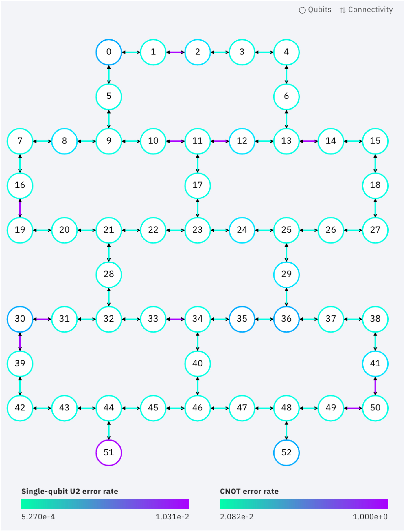
For Melbourne it is possible to find a line that covers all 15 qubits. The choice one specified in the list line below is designed to avoid the most error prone cx gates. For the 53 qubit Rochester device, there is no single line that covers all 53 qubits. Instead we can use the following choice, which covers 43.

Now we know how many qubits we have access to, we can create the repetition code objects for each code that we will run. Note that a code with n repetitions uses n code qubits and n − 1 link qubits, and so 2n − 1 in all.

Before running the circuits from these codes, we need to ensure that the transpiler knows which physical qubits on the device it should use. This means using the qubit of line[0] to serve as the first code qubit, that of line[1] to be the first link qubit, and so on. This is done by the following function, which takes a repetition code object and a line, and creates a Python dictionary to specify which qubit of the code corresponds to which element of the line.

Now we can transpile the circuits, to create the circuits that will actually be run by the device. A check is also made to ensure that the transpilation indeed has not introduced non-trivial effects by increasing the number of qubits. Furthermore, the compiled circuits are collected into a single list, to allow them all to be submitted at once in the same batch job.

We are now ready to run the job. As with the simulated jobs considered already, the results from this are extracted into a dictionary raw_results. However, in this case it is extended to hold the results from different code sizes. This means that raw_results[n] in the following is equivalent to one of the raw_results dictionaries used earlier, for a given n.

It can be convenient to save the data to file, so that the processing of step (c) can be done or repeated at a later time.

As was described previously, some post-processing of the syndromes is required to find the graph that will be used in the decoding. This is done using the process_results method of each repetition code object code[n]. Specifically, we use it to create a results dictionary results[n] from each raw_results[n].

The decoding also needs us to set up the GraphDecoder object for each code. The initialization of these involves the construction of the graph corresponding to the syndrome, as described in the last section.

Finally, the decoder object can be used to process the results. Here the default algorithm, minimum weight perfect matching, is used. The end result is a calculation of the logical error probability. This is simply the probability that the decoded output is 1 when the encoded value was 0, or vice-versa.
When running step (c), the following snippet also saves the logical error probabilities. Otherwise, it reads in previously saved probabilities.

The resulting logical error probabilities are displayed in the following graph, which uses a log scale on the y axis. We would expect that the logical error probability decays exponentially with increasing n. If this is the case, it is a confirmation that the device is compatible with this basis test of quantum error correction. If not, it implies that the qubits and gates are not sufficiently reliable.
Fortunately, the results from this device does show the desired trend. Deviations can be observed, however, which can serve as a starting point for investigations into exactly why the device behaves as it does. However, in this paper we simply seek to show an example of the topological_codes module in action, and will not perform more in-depth analysis.

Another insight we can gain is to use the results to determine how likely certain error processes are to occur. To see how this can be done, recall that each node in the syndrome graph corresponds to a particular syndrome measurement being performed at a particular point within the circuit. A pair of nodes are connected by an edge if and only if a single error, occurring on a particular qubit at a particular point within the circuit, can cause the value of both to change.
For any such pair of adjacent nodes, we will specifically consider the values C11 and C00, where the former is the number of counts in results[n]['0'] corresponding to the syndrome value of both adjacent nodes being 1, and the latter is the same for them both being 0.
The most likely cause for each event recorded in C11 is the occurrence of the error corresponding to the edge between these two nodes. Also, it is most likely that this error has not occurred for each event recorded in C00. As such, to first order, we can state that

Where p is the probability of the error corresponding to the edge between these two nodes.
For example, suppose that one of the nodes we are considering corresponds to the syndrome measurement of code qubits 0 and 1 in the first round, and the other corresponds to the same for code qubits 1 and 2. If both syndrome measurements output 0, it is most likely that none of these three qubits suffered an error (during the initial state preparation or during the controlled-NOTs required for the syndrome measurements). If both syndrome measurements output 1, it is most likely that a single error occurred on the shared qubit 2. The probability p in this case would therefore be that for such an error on qubit 2, either in preparation or during the controlled-NOTs.
The decoder object has a method weight_syndrome_graph which determines these ratios, and assigns each edge the weight −ln(p/(1 − p)). By employing this method and inspecting the weights, we can easily retrieve these probabilities.

count: 85.0
mean: 0.150 194 280 998 097 15
std: 0.112 369 952 059 353 89
min: 0.026 545 002 073 828 285
25%: 0.055 994 503 607 007 91
50%: 0.111 558 598 469 593 23
75%: 0.202 860 061 287 027 58
max: 0.416 297 117 516 629 73
These probabilities come from a novel way of benchmarking the device, that is distinct from currently used methods. Since no other set of available error probabilities are exactly equivalent, it is not possible to do a direct comparison. Nevertheless, since the results from the standard benchmarking of the device can be easily obtained from the backend object, we will generate a similar summary. Specifically, we will look at the readout errors and controlled-NOT gate errors.

count: 127.0
mean: 0.068 501 611 544 310 56
std: 0.058 911 713 612 484 07
min: 0.019 374 999 999 999 92
25%: 0.037 087 748 989 323 93
50%: 0.046 021 125 148 897 085
75%: 0.085 753 643 214 1715
max: 0.336 249 999 999 999 94
Note that, despite the different methods used to obtain these values, there is excellent agreement for the minimum and first quartile. However, the values from the repetition code do show more of a skew to larger values in the upper quartiles. This could be due to the fact that repetition code values are obtained from an approximation that is less accurate for higher error probabilities. The possibility of using a better approximation will therefore be investigated in future versions of topological_codes, as will further study of how the results of this benchmark relates to the standard one.
4. Conclusions
In this paper we have provided an introduction to the repetition code and its implementation in Qiskit. It forms part of the topological_codes module of Qiskit-Ignis. This module has been designed to have a modular form, allowing new codes and decoders to be added with relative ease. It will be expanded to include more codes, such as the 17 qubit variant of the surface code [25, 26]. It will also be expanded to introduce new decoders, such as Bravyi–Haah [27] and methods devised as part of the 'Decodoku' citizen science project [28]. There are also many other possible ways to expand the module. One aim of this paper is to serve as a starting point for anyone interested in making any contributions to this open-source project.
Results were shown from an example run from a 43 qubit code running on IBM's Rochester device. This showed what can be done using just a few lines of code. However, much more could be done to fully probe the working of a device using the repetition code. The most obvious would be to use different possible choices for line, to fully map out where the errors come from and what effect they have. This paper also serves to serve as a starting point for such endeavours, since anyone with an internet connection can now use the tool to probe the 15 qubits of IBM's publicly accessible Melbourne device.
Acknowledgments
This paper was based on resources developed for the Qiskit tutorials and textbook [29]. The author would therefore like to thank all members of the Qiskit Community.