

Abstract
Small-scale farming provides both food and livelihoods for the vast majority of the global poor. Thus, increasing and stabilizing farm incomes and food production in developing countries is fundamental to reducing global poverty. Policies for rural development such as improved access to non-agricultural incomes or land titling may benefit farmers, but they may also lead to farm consolidation with unintended consequences for aggregate food supply. Using a large panel dataset of rural households in Uganda, we parse apart how farm size affects the level and riskiness of agricultural incomes as well as of local food supply. Our findings indicate that while output per unit of land does decline with increasing farm size as suggested by previous literature, agricultural incomes increase with farm size. We show further that while the variance of agricultural incomes declines with increasing farm size, the variance of local food production increases with farm size. These results suggest that farmers benefit from larger farms, earning higher and more stable incomes while consumers suffer from lower and more volatile food supply.
Export citation and abstract BibTeX RIS

Original content from this work may be used under the terms of the Creative Commons Attribution 3.0 licence. Any further distribution of this work must maintain attribution to the author(s) and the title of the work, journal citation and DOI.
Introduction
Despite the increasing share of the poor in urban areas, global poverty is still predominantly a problem of low agricultural incomes in rural areas of developing countries (World Bank 2016). While many development agencies have sought to reduce yield gaps through improved access to technologies, the potential to raise small farm incomes through productivity gains is, however, largely limited by the small farm sizes. For example, Adamopoulos and Restuccia (2014) find that more than 70% of the farms in poor countries are less than 2 hectares. For these farms it may not be sufficient to increase farm productivity in order to lift farmers above the poverty line. As such, much research in development economics has focused on improving access to non-farm incomes (Jensen 2012, Blattman et al 2013, Bryan et al 2014). However, improving rural poverty through reduced on-farm labor may have unintended consequences for regional food production and food security.
Access to non-agricultural employment and rural–urban migration implies less labor allocated to agriculture. This reallocation of labor may harm low-income consumers who depend on the availability and stability of affordable locally produced food. Small scale agriculture produces 70% of the food calories in developing countries (Samberg et al 2016). Further, the dependence on local agriculture is especially strong in developing countries where high trade costs impede trade of agricultural goods with neighboring countries (Porteous 2019). Thus, a reduction of food production as a consequences of labor reallocation may have severe consequences for poor consumers.
The process of labor reallocation from agriculture to non-agriculture has led to farm consolidation and rural prosperity in most developed countries. However, a large literature studying the relationship between farm size and productivity generally concludes that farm output declines with farm size in most developing countries (Bardhan 1973, Carter 1984, Feder 1985, Benjamin 1995, Assuncao and Braido 2007, Barrett et al 2010, Carletto et al 2013, Ali and Deininger 2015, Foster and Rosenzweig 2017), though concerns about measurement error have plagued consensus (Gourlay et al 2017, Desiere and Jolliffe 2018, Gollin and Udry 2019). The implication of an inverse farm size-productivity relationship for consumers is that food supply declines with increasing farm size. The transition to non-agricultural employment and larger farms may therefore harm consumers of agricultural goods in developing countries. Although there is a large overlap between consumers and producers in developing countries we use these terms to refer to net consumers and net producers in the following. Although studies have considered the trade-offs between consumers and producers from higher food prices (Byerlee et al 2006, Aksoy and Isik-Dikmelik 2008, Ivanic and Martin 2008), very little is known about the implications from changing farm size distributions for those who work in agriculture and those who depend on agriculture for consumption.
Farmers and consumers of agricultural goods in developing countries not only suffer from chronic poverty but they often experience income shortfalls and food price spikes due to droughts, pest outbreaks or crop diseases causing large scale agricultural failures. These agricultural shocks can lead to conflict and civil unrest when poverty and malnutrition become rampant (Couttenier and Soubeyran 2014, von Uexkull et al 2016, Crost et al 2018, Harari and La Ferrara 2018). Larger farms may operate under different economic constraints and can hedge differently against risk compared to smaller farms (Rosenzweig and Binswanger 1993). For example, they may leverage their larger farms to diversify their risks by planting more or different crops. Larger farms may not benefit producers and consumers likewise. In contrast to producers, the risk of food supply for consumers also depends on the covariance of production across farms. In other words, the covariance of production across farms may depend on the size of the farms as fewer and larger farms potentially have more similar access to technologies, grow more similar crops, and thus have more similar outcomes than a large number of small farms. Even if the covariance of production is unaffected by farm size, a large number of small farms may still supply more stable food by diversifying risk, just as a larger number of stocks in a portfolio of an investment manager or more species in an ecosystem reduces the variance of the returns or biomass production. Despite the importance of agriculture for rural poverty and food security, the relationship between farm size and the stability of rural incomes and food supply is largely unknown.
In the current study, we shift the discourse from the farm size-productivity relationship to ask how changes in farm size affect the welfare of both producers and consumers taking the individual and aggregate risk of production explicitly into account. Specifically, we address the question of how farm size affects (1) the level and stability of agricultural incomes and (2) the level and stability of food supply. Like the previous literature on the farm size-productivity relationship, we focus on the impact of farm size, neglecting the multiple drivers of farm size changes that may also affect production directly. This paper further contributes to this literature by addressing the endogeneity problem of farm size and by including consumption as an alternative welfare measure that is independent of the measurement error of production. In our study, we focus on Uganda, where like in most rural parts of Africa and Asia, rural poverty persistently high, agricultural productivity is persistently low and agriculture is dominated by a large number of small farms. Using a combination of panel data and instrumental variables techniques informed by a conceptual model, we identify the effect of farm size on the level and stability of income and food supply after overcoming statistical concerns regarding heterogeneity in farmer, household and land characteristics, measurement error in self-reported farm size, as well as the potential that farm size is endogenously determined with productivity. To further address the problem of measurement errors in self-reported production, we use household consumption data to confirm our results. Our empirical findings suggest that while output per unit of land declines with increasing farm size the reverse is true for farmer income and consumption. Further, we find that the riskiness or variability of farmer incomes and consumption declines with farm size. This unambiguously positive result for farm size and rural income is reversed for food supply at the aggregate level. Our results therefore suggest that farmers in Uganda benefit from larger farms, earning higher and more stable incomes, while consumers suffer from lower and more risky food supply.
Data
For our empirical analysis, we use the data of the Living Standards Measurement Study-Integrated Surveys on Agriculture in Uganda (LSMS-ISA). The LSMS-ISA data are plot level information on seasonal crop production including data on crop type, inputs and other production practices, and yields. The survey is composed of structured interviews of ∼3200 households chosen based on the stratified random sample of the Uganda National Household Survey in 2005/06. Interviews were conducted in four rounds between 2009/10 and 2013/14 with visits in each of the two growing seasons per year. However, we include the initial survey of 2005/06 as well but exclude the urban stratum to focus on the rural production, which results in a sample of 13 368 complete household and season level observations. The survey design is described in detail in the appendix A and on the LSMS-ISA webpage.
Our key variables were farm size, labor, land productivity, output and income. We define farm size as the sum of land that is currently cultivated by the farm including land under fallow but excluding land under natural vegetation, trees or pasture. The reason for including fallow but excluding natural vegetation is that fallow is an investment in soil quality which increases agricultural productivity while natural vegetation could indicate either physical or legal land use restrictions. In a robustness check we also include land under natural vegetation, trees or pasture in our farm size measure (appendix C.3). Labor is defined as the sum of days worked by family members on the farm plus days of hired labor. Output is defined as production, provided by the farmer in local units. We convert these units to kilograms (kg) using the median district level conversion factors from the survey, and use prices and calories to aggregate yields across crops. Crop specific caloric values were derived from the Food Balance Sheets of the Food and Agricultural Organisation. To compute revenues we follow Restuccia and Santaeulalia-Llopis (2017) using median crop level prices and subtracting variable costs such as fertilizer and pesticide costs (which were negligible here). Income is defined as output per unit of labor (see appendix B for the theoretical background of this measure). The variables are summarized in the descriptive statistics in appendix A.
As is common in survey data, there is a concern with recollection bias in measures of our key variables. For example, self-assessed land sizes with small plots are generally overestimated (Dillon et al 2019, Sheahan and Barrett 2017). To address this concern, we used GPS measured field sizes to confirm self-assessed land sizes. We corrected for overestimation of small fields and underestimation of large fields observed in our sample as well as the knock-on effects of over/underestimation of field size on farm size (appendix A). Additionally, farms on less productive land may be larger such that measuring farm size in hectares may overestimate differences in effective farm sizes. We address this concern using household fixed effects (household dummies) in our main specification. In a second specification we weight farm size by median farm level self-assessed land values to account for land productivity differences across farms. Prices for agricultural land reflect land productivity directly. Estimated land values are stated by the farmers for several of their fields. Additionally, there is a growing concern about recollection bias of rural production (Gourlay et al 2017, Desiere and Jolliffe 2018, Gollin and Udry 2019). To test the robustness of the relationship between farm size and incomes we use household consumption of food and beverages as alternative welfare measure for producers. While consumption is generally seen as a robust alternative to incomes as welfare measure (Meyer and Sullivan 2003) the same holds true for food consumption in areas such as Sub Saharan Africa where households spends the largest share of their incomes on food (De Magalhães and Santaeulàlia-Llopis 2018).
Estimation
In the appendix we develop a simple theoretical framework to guide our estimation strategy (see appendix B). Based on our theoretical results and using the two-step procedure by Just and Pope (1978) we estimate the impact of farm size on the level of output in a first stage and the impact of farm size on the variance of production using the residuals from the first stage in a second stage. Just and Pope's main innovation was to interpret the error term of a first stage regression as the risk of production. In other words, a heteroskedastic error term can be interpreted as an impact of inputs on the risk of production. We use ordinary least squares (OLS) to estimate the parameters in this two-step procedure but compare the results to an alternative approach in which we estimate the mean and the variance of production simultaneously using a multiplicative heteroskedastic linear regression framework based on maximum likelihood estimation (Harvey 1976). In our main specification, we estimate the impact of farm size on the level and the risk of production, estimating

in a first stage and
in a second stage, where  denotes the output of farmer i in district j and region k at time t measured both in revenues and calories per unit of land in one specification and per unit of labor in the second specification. The variable
  denotes farm size while
  is the heteroskedastic error of the first stage regression and
  is the error term of the second stage which is related to the random component of the first stage error term.
The parameters  and
and  are household level fixed effects (dummies), which absorb household-specific characteristics such as time constant differences in land quality and farmer skill levels while
  and
and  are region specific year-season fixed effects (dummies) to account for region-specific seasonality, time trends and shocks such as climate change, droughts or heat waves. Our main specification is therefore identified from the intertemporal variation in farm size and output of individual farms that differ from regional averages. The parameter
  captures the total factor productivity differences across farm e.g. the fact that some farmers can convert the same amount of inputs into more output than others.
Independent of input market functioning, a parameter estimate of  implies that log output per unit of land or labor declines with farm size while
  implies that the risk of production declines with farm size (see appendix B). Generally, we expect output per unit of land to decline faster with increasing farms size under malfunctioning input markets as households are unable to adjust other inputs such as capital and labor to increasing land sizes.
The main concern for our empirical strategy is that farm size may be endogenous. First, farm size may depend on farmer skills which could also determine output. We account for the time constant skill differences by household fixed effects. These household level fixed effects also capture average differences in soil quality and climate across farms. Still, farm size may change in response to household productivity dynamics such as sickness and changes in the household composition that could also drive changes in output. To test the endogeneity of farm size we use inherited land as an instrument for farm size. Inheritance of land is outside of the household's control and therefore fulfills the exclusion restriction for instrumental variables. 30% of our households inherited land during the survey period from 2005 to 2013 allowing us to use inherited land as instrument in combination with household fixed effects.
To account for the heteroskedasticity and the correlation of error terms within clusters, we use heteroskedasticity robust standard errors clustered at the district level (Cameron et al 2011). In a robustness test, we further estimate the impact of farm size on the mean and the variance of production simultaneously using a multiplicative heteroskedastic linear regression framework. The results are reported in appendix C.1.
To assess the impacts of farm size on aggregate production we sum farm level production per district, and estimate the impact of the log number of farms and the log size of total farmland on the level and variance of output. Estimating the impact of the log number of farms and the log aggregate land size on output is mathematically equivalent to estimating the impact of mean farm size on output but it allows us to separate the impact of spatial heterogeneity or the covariance across fields (captured by aggregate land size) from the impact of covariance across farms (captured by farm numbers) on the risk of aggregate food production. For our purpose it is not important if the aggregate production comprises all farms in the district (it does not) or even if the sample is representative at the district level. Instead, we are interested in the impact of farm size on aggregate production of a random sample of farms (see appendix B). Generally, we follow the same estimation procedure as for the farm level without household level fixed effects but with region-season-year fixed effects.
Results
To understand how farm size affect producers and consumers we start with a visual analysis of the data. Figure 2 shows that output and labor per unit of land decline with farm size (figures 2(A) and (B)) which implies that overall agricultural production declines with increasing farm size. However, labor declines faster than output per unit of land such that the output per unit of labor increases with increasing farm size (figure 2(C)). The latter finding implies that agricultural incomes increase with farm size independent of market functioning (see appendix B). These relationships therefore suggest that agricultural production declines with farm size with negative consequences for consumers while agricultural incomes increase with farm size with positive benefits for producers.
The results of our first regression specification (DI) using district level fixed effects (dummies) and additionally season-region-year specific fixed effects to control for local seasonality, weather and price shocks confirms these visual pattern (figures 3(A) and (B)). In this first regression specification, we use the variation across farms to estimate our parameters with the advantage that we not only rely on farm expansion or on contraction to estimate the relationships but also with the disadvantage that unobserved differences across farms may bias our results. The results of this specification suggest that a one percent increase of farm size reduces output per unit of land by 0.18% but increases output per unit of labor by 0.22%. These relationships are not statistically different between the specifications that measure output in revenues (blue in figure 3) and the specifications that measure output in calories (gray in figure 3). Weighting farm size by farm level land value estimates (Ush), which reflect land productivity and therefore convert farm size from physical units to effective units, suggest that the negative effect of farm size on output per unit of land is stronger after accounting for productivity differences of land (figures 3(A), (B)).
Still, the relationship between farm size and income could be driven by farmer skills, which may not be reflected in land prices. However, our results show that including household fixed effects, which account for roughly time invariant characteristics of the household such as farmer skill and soil quality (see methods), does not change the magnitude of the estimates. This suggests that differences in land productivity have a stronger impact on agricultural production than does farmer skill (figure 1).
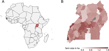
Figure 1. The figure shows (A) the location of Uganda within Africa and (B) the farm size distribution within Uganda on district level.
Download figure:
Standard image High-resolution imageThe relationship would have no causal interpretation if both farm size and outcomes are driven by an omitted third variable. Yet, the estimates from the IV regression are qualitatively similar to our main specification (Model HH), suggesting that the endogeneity of farm size does not bias our estimates. In an alternative IV approach, we use only land inheritance instead of the amount of inherited land as instrument in combination with household fixed effects. In this specification, the estimates for the impact of farm size on output per unit of land are −0.64 (p < 0.05) and −0.72 (p < 0.05) for revenues and calories respectively. The estimates for the output per unit of labor are statistically insignificant as the precision of the IV estimate is low despite strong instruments (the F statistic is 117 and 55 respectively).
Market access may differ between small and large farms. To account for this possibility, we estimate the regression specification with household fixed effects (HH) separately for the sample of the 25% of the largest and the 25% of the smallest farms (not shown in figure 1). The results show that an increase of farm size by one percent reduces output per unit of land by 0.56% for the smallest farms (−0.55 ± 0.10***) while it reduces output per unit of land by 0.74% for the largest farms (−0.74 ± 0.11***). The results show further that the difference in the relation between farm size and incomes between small and large farms is negligible (−0.16 ± 0.10 for small farms and −0.17 ± 0.08* for large farms). These results therefore suggest that larger farms in our sample do not have better access to input markets since better markets access would imply smaller impacts of farm size on production and therefore smaller coefficients estimates in absolute terms.
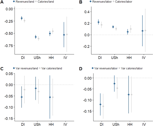
Next, we discuss our results on the relationship between farm size and the variance of production. All regression specifications are as defined earlier but instead of log output we use the log of the squared residuals from the first stage regression as the dependent variable (figures 3(C) and (D)). Here, the coefficients measure the impact of a percentage change of farm size on a percentage change of the variance of production. We do not interpret the variance of the IV estimate since it contains errors from the first stage of the IV estimation. The results from the other model specifications show that the estimates are negative, although not always statistically significant. For our main specification (HH) the estimates are −0.07 (p > 0.05) for the impact of farm size on the variance of output per unit of land (both calories and revenues) and −0.07 (p < 0.05) for the impact of farm size on the variance of output per unit of labor (both calories and revenues) (figures 2(C) and (D)). These results imply that farm size reduces the risk of agricultural incomes and of output per unit of land although the latter effect is not statistically significant. Another important measure of risk is the coefficient of variation i.e. the variance divided by the mean. When risk is measured by the coefficient of variation instead of the variance, the risk reducing effect of farm size on agricultural income increases further because of the simultaneous positive impact of farm size on agricultural incomes and the negative impact of farm size on the variance of agricultural incomes.
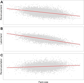
Figure 2. Shows a scatter plot and a linear regression line of (A) log revenues per unit of land and log farm size, (B) log labor per unit of land and log farm size and (C) log revenues per unit of labor and log farm size. All variables are standardized at the district—season—year level and farm size is measured in land value.
Download figure:
Standard image High-resolution imageThe precision of the estimates increases when we estimate the impact of farm size on the mean and the variance of production simultaneously using a maximum likelihood estimator but the results are qualitatively similar (see appendix C.1).
To further test the robustness of our results on the impact of farm size on farm income, we estimate the same models as above but with farm consumption as dependent variable. The results are reported in the appendix C.2. Overall, the estimates are remarkably similar to those with farm income as dependent variable reported in figure 3. We interpret these results as evidence for a relationship between farm size and agricultural production independent of the measurement of production.
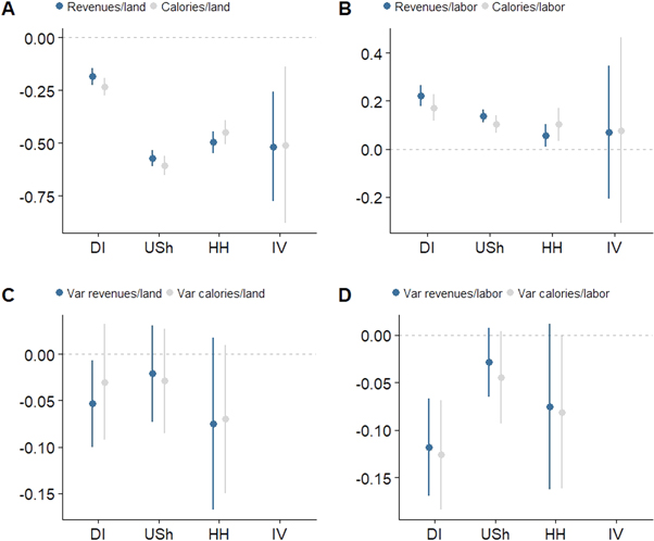
Figure 3. Marginal effects (elasticities) of farm size on the mean and the risk of production measured in revenues (blue) and calories (gray). Outcomes are (A) log production per hectare, (B) log production per unit of labor, (C) variance of log production per hectare and (D) variance of log production per unit of labor. The variance of the IV specification also contains the errors from the first stage regression of farm size on inherited land and cannot be interpreted in the same way. It is therefore omitted from the figure. Model specifications are DI: OLS with farm size in hectares and district fixed effects, USh: OLS with farm size in monetary value (USh) and district fixed effects, HH: OLS with crop land in hectares and household fixed effects and IV: instrumental variable regression with crop land in hectares, household fixed effects and inherited land as instrument for crop land. All regression specifications include region specific season and year fixed effects (dummies). Standard errors are heteroskedasticity robust and clustered at the district level.
Download figure:
Standard image High-resolution imageConsumers rarely rely on the production of an individual farm. Instead, they mostly buy food from a portfolio of farms within a larger region. To estimate the impact of farm size on the level and riskiness of aggregate food supply, we estimate the impact of farm numbers and aggregate land size (the sum of farm sizes) on aggregate output. The results at the district level (table 1) confirm our results from the farm level analysis. An increase of total farmland by 10% for a given number of farms reduces output per unit of land by 2% (revenues) to 3% (calories) if land is measured in physical units or by 7% (revenues) to 9% (calories) if land is measured in monetary units. Note, however, that this implies an increase of aggregate production by 1%–8% depending on the specification since the coefficient measures the elasticity of aggregate output minus one. Increasing the number of farms for a given amount of land has an even larger impact on production. An increase of farm numbers by 10% increases output per unit of land by 4% to 5% if land is measured in physical units and between 10% and 11% if land is measured in monetary units. These results are qualitatively similar to the results on the impact of farm size on the output per unit of land on farm level reported in figure 3.
Table 1. Impact of the number of farms and on district level crop production.
| R1 | C1 | R2 | C2 | |
|---|---|---|---|---|
| Log farmland | −0.20* | −0.31*** | −0.77*** | −0.91*** |
| (0.12) | (0.12) | (0.07) | (0.06) | |
| Log farm number | 0.41*** | 0.51*** | 1.01*** | 1.15*** |
| (0.15) | (0.14) | (0.09) | (0.10) | |
| Observations | 712 | 712 | 712 | 712 |
| R2 (full model) | 0.46 | 0.96 | 0.64 | 0.89 |
Notes. The dependent variable is log output per unit of land at the district level measured in revenues (R1 and R2) and calories (C1 and C2). The independent variables are log total land and log farm numbers. All specifications include region fixed effects and region specific year and region specific season fixed effects (dummies). Specifications R1 and C1 measure farm size in land area while specifications R2 and C2 measure land in land value. Standard errors are heteroskedasticity robust. Significance levels are ***p < 0.01, **p < 0.05, *p < 0.1.
The results for the risk of production at the district level reverse, however, from the results at the farm level. At the district level, dividing the total farmland among more farms reduces the variance of production per unit of land (table 2). A 10% increase of the number of farms reduces the variance of log revenues by 3%–7% depending on measuring the land either in physical or monetary units. The same increase of farm numbers reduces the variance of calorie supply by 3% independent of the land measure. These results suggest that raising farm numbers for a given amount of farmland has a large impact on the risk of aggregate production. In contrast, an increase of farmland for a given number of farms has no statistically significant impact on the risk of aggregate production. These results suggest that dividing production among more farms (not all eggs in one basket) drives the result.
Table 2. Impact of farm size on the variance of district level crop production.
| R1 | C1 | R2 | C2 | |
|---|---|---|---|---|
| Farmland | 0.19 | −0.08 | −0.05 | −0.03 |
| (0.23) | (0.25) | (0.11) | (0.09) | |
| Farm number | −0.71*** | − 0.32 | −0.34** | − 0.26* |
| (0.26) | (0.27) | (0.17) | (0.15) | |
| Num. obs. | 712 | 712 | 712 | 712 |
| R2 (full model) | 0.17 | 0.17 | 0.14 | 0.10 |
Notes. The dependent variable is the log variance of the log output per unit of land at the district level measured in revenues (R1 and R2) and calories (C1 and C2). The independent variables are total land and farm numbers. All specifications include region fixed effects and region specific year and season fixed effects (dummies). Specifications R1 and C1 measure land in physical units while specifications R2 and C2 measure land in monetary units. Standard errors are heteroskedasticity robust. Significance levels are ***p < 0.01, **p < 0.05, *p < 0.1.
We present results on aggregate production but with district fixed effects in appendix C.3. They are, however, qualitatively, similar to the results presented above.
Discussion
Reducing global poverty and increasing global food security are among the Sustainable Development Goals of the United Nations. Both goals concern mainly rural areas in developing countries where poverty is widespread and agricultural productivity is low. Recent studies suggest that improving income alternatives of the rural poor can alleviate rural poverty and lead to improved development outcomes (Blattman et al 2013, Bryan et al 2014). However, these policies may also cause rural–urban migration and farm consolidation with potentially far reaching consequences for local food supply.
Here, we sought to understand the implications of increasing farm size on farmer and consumer well-being. Our results show that farmers earn higher and more stable incomes with increasing farm size while consumers suffer from lower and more variable food supply. More specifically, increasing farm size reduces the output per unit of land but larger farms have higher output per unit of labor. Further income fluctuations decline with increasing farm size while the risk of aggregate production increases with increasing farm size. The effects can be large. Increasing the median farm size in 2013 from 0.9 to 1.8 hectare would approximately reduce output per unit of land by 50%, increase farm income by 5% and reduce farm income variance by 8% using the parameter estimates of our preferred specification (HH) with household fixed effects. Although the estimated impact of farm size on output per unit of land is large, our estimate is similar to findings from comparable studies (e.g. Barrett et al 2010, Carletto et al 2013, Ali and Deininger 2015). At the aggregate level and under the assumption that the total land is constant, the same change of farm size implies that the variance of aggregate food supply increases by 30% using the parameter estimate of our preferred specification (R2) reported in table 2. These large numbers illustrate the magnitude of the trade-off between farmer and consumer welfare.
It is not possible to derive a socially optimal farm size distribution from our results without further information for several reasons. First, reducing average farm size would increase and stabilize agricultural production and therefore benefit consumers but simultaneously, it would reduce and destabilize agricultural incomes. The welfare maximizing farm size distribution depends therefore on the wealth distribution within the society and the possibility of wealth transfers between consumers and producers as well as the alternative income options of farmers and the access to international food markets of consumers. Second, we have ignored productivity differences across farms resulting from skill differences (see e.g. Adamopoulos and Restuccia 2014). The household fixed effects in our main specification capture these differences. However, welfare maximizing land allocations would consider skill levels and may therefore result in very unequal farm size distributions. Third, most farmers have additional non-farm income and buy food to compliment their own agricultural production for consumption. Most producers are therefore also consumers who buy agricultural goods on markets. The magnitude of the welfare effect therefore depends on consumption relative to production and differs within the group of net consumers and net producers. However, the direction of the effect within one group is homogeneous (positive or negative).
Our findings suggest that malfunctioning labor market drive the results. This reflects that 90% of labor in agriculture is family labor in our data. The findings therefore suggest that larger farms are not necessarily less productive but that they use less inputs per unit of land. The implication of our finding is that improving rural input markets (mainly labor and land) would solve the problem of the negative relationship between yields and farm size.
The magnitude of the negative impact of larger farms on local consumers depends on consumers' access to global markets for food. Improved access to international food markets can mitigate the problem of reduced local food supply and increased volatility of food production but may harm local producers who would face increased competition.
Alleviating rural poverty is a fundamental societal goal. One common means of doing so, access to non-farm income, has spurred concerns about worsening already fragile food systems. Here we show that productivity is only one aspect. Rather, rural incomes both increase and stabilize as farm size increases, an unambiguous positive for poor farmers. However, our results caution that policies supporting farm consolidation can have negative consequences for consumers. Other policies such as the provision of improved technologies or better access to credit markets to support technology adoption can increase farmer incomes and food production simultaneously.
Appendix A.: Data
Appendix. A.1. Living standards measurement study-integrated surveys on agriculture in Uganda
For our empirical analysis, we use the data of the LSMS-ISA. The LSMS-ISA data are plot level information on seasonal crop production including data on crop type, inputs and other production practices, and yields. The survey is composed of structured interviews on ∼3200 households chosen based on the stratified random sample of the Uganda National Household Survey in 2005/06. We combine the data of the LSMS-ISA with the Uganda National Household Survey in 2005/06 to extend the time span that the survey covers.
Interviews were conducted in four rounds between 2009/10 and 2013/14 with visits in each of the two growing seasons per year. We exclude the urban stratum to focus on the rural production, which results in a sample of 13 368 complete household and season level observations. Each year, a random sample of the previous year was re-interviewed while the other fraction was replaced by newly sampled households. Households in the sample were tracked and re-interviewed. About 50% of the households that were interviewed in 2005/06 were also present in the survey of 2013/14. The survey is representative at the national, urban/rural and regional level (http://surveys.worldbank.org/lsms/integrated-surveys-agriculture-ISA/uganda).
As household were randomly sampled, we use the unbalanced panel for our empirical analysis.
Appendix. A.2. Markets
In our sample, about 60% of the land is in customary tenure while only about 30% of the land has formal land titles. The remaining 10% of the land in our sample is in leasehold or other forms of tenure. However, even the existing land titles do not guarantee secure ownership over the land (Baland et al 2007). As a consequence, the most common type of transfer in our sample is inheritance between father and sons (64%) while market transactions account only for 32% of the land transfers. Clearing of previously unoccupied land is relatively rare and accounts for 2% of the transfers. Labor markets are even less developed than land markets. About 90% of the farm labor is family labor. The percentage of hired labor increases from 8% for the smallest farm quintile to 17% of the largest farm quintile suggesting that larger farms participate more in markets. Output markets are also little developed. Only 23% of the agricultural products are sold while the remaining 77% are consumed by the farmers themselves. The share of the production that is sold slightly increases from 18% for the smallest farm quintile to 28% for the largest farm quintile.
Appendix. A.3. Farm size correction
To test for potential bias in stated field sizes we estimate

where  is the plot size measured by GPS signal and
  is the plot size stated by the farmer. The point estimate with standard errors clustered at the district level is
  which indicates an overestimation of small fields (or an underestimation of large fields). As field size generally increases with farm size in our sample, our estimates of farm sizes are biased. To correct for this bias, we use predicted field size,
  in our regression specification using the relationship

We use the corrected farm size instead of the GPS measurements directly because they are only available for about 60% of the fields.
Appendix. A.4. Farm size distribution
Figure A1 shows the farm size distribution within Uganda in 2005 and 2013. In contrast to most regions of the world, median farm size has declined in Uganda from 1.3 ha in 2005 (mean 1.7 ha) to 0.9 ha (mean 1.1 ha).
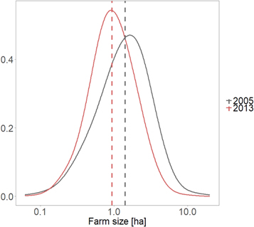
Figure A1. Farm size distribution and median farm size (dashed line) in Uganda in 2005 (grey) and 2013 (red).
Download figure:
Standard image High-resolution imageAppendix. A.5. Summary statistics
Table A1 provides the summary statistics for the key variables.
Table A1. Summary statistics.
| Mean | Max | Min | St. Dev. | Median | Q25 | Q75 | |
|---|---|---|---|---|---|---|---|
| Farm size (ha) | 1.4 | 53 | 0 | 1.5 | 1.0 | 0.6 | 1.7 |
| Labor (d) | 139 | 3462 | 0 | 130 | 108 | 60 | 179 |
| Revenues (106 USh) | 0.8 | 361 | 0 | 5.1 | 0.3 | 0.1 | 0.7 |
| Calories (106) | 2.9 | 2163 | 0 | 25 | 1.0 | 0.3 | 2.5 |
Notes. Q25 and Q75 are the 25th and 75th percentiles respectively. The numbers are rounded to one decimal place for all values below 10 and to the nearest integer for values above 10.
Appendix B.: Theoretical framework
In the following, we develop a simple theoretical framework to motivate our empirical approach, to produce testable predictions and to guide the interpretation of the results. Within this framework we discuss (a) the impact of farm size on output per unit of land under different scenarios of factor market functioning, (b) the relation of output to agricultural incomes and (c) the framework to estimate the risk of production on individual and aggregated level. The framework is generally based on the work by Just and Pope (1978, 1979) on risk and agricultural production.
Consider a farmer producing crops using labor, capital and land. Agricultural production is stochastic and we assume a log normal distribution of outputs. Assuming a standard Cobb–Douglas production function we can represent production by

where A is the total factor productivity, L is labor, K is capital, X is land,  is a positive number and
  is a standard normal stochastic term with
 ![$E[\varepsilon ]=0$](https://content.cld.iop.org/journals/1748-9326/14/8/084024/revision2/erlab2dbfieqn18.gif) and
and ![$E[{\varepsilon }^{2}]=1.$](https://content.cld.iop.org/journals/1748-9326/14/8/084024/revision2/erlab2dbfieqn19.gif) Total factor productivity may depend on farmer skills, the environment such as weather conditions and technology levels. To simplify notation we assume further that it contains the vector of prices or nutritional values. The constant
Total factor productivity may depend on farmer skills, the environment such as weather conditions and technology levels. To simplify notation we assume further that it contains the vector of prices or nutritional values. The constant  represents the standard deviation of
  Although the production technology is very specific, we think that our qualitative results apply to all homogeneous production functions (such as e.g. CES functions) and all homothetic transformations such as risk averse utility functions over productions. The key property of these functions driving our results is that all variable production factors are used in constant proportions such that inputs can be expressed as linear functions of each other.
Appendix. B.1. Farm size and output
For perfectly functioning input markets, optimality requires that
where  denotes the respective input prices. Dividing the first order condition for land by the first order condition for labor and capital respectively yields

and

Inserting these expressions into the production function yields
 where
where  is a composite parameter of total factor productivity, relative input prices and factor intensities (the alphas). Constant returns to scale technologies implies
  such that total output scales with farm size i.e. a doubling farm size also doubles production. Dividing both sides by farm size, X, yields the output per unit of land

For constant returns to scale technologies the output per unit of land is given by the constant  However, the finding that output decreases with farm size hints at decreasing returns to scale technologies and therefore
  A second possible explanation for the negative relationship of farm size and output is malfunctioning input markets. In fact, if factor markets are missing, production factors are determined by the household endowments and equation (A2.1) can be written as

where  is composed of total factor productivity and factor endowments of the household (the size of the labor force and capital endowments).
For absent land markets but perfectly functioning capital and labor markets the first order condition for land drops out. However, rearranging the first order condition for capital and labor yields
Inserting these expressions into each other and then into the production function yields

Note that  such that output declines always faster with farm size if factor markets are missing or malfunctioning, compared to the perfect market scenario.
Appendix. B.2. Farm size and agricultural incomes
Output per unit of land is mainly important for consumers as higher supply is expected to decrease prices which makes food more affordable. However, many studies find a wage gap between the rural and the urban population (Gollin et al 2013). The wage gaps suggest that the rural population is poorer than the urban population which implies that reducing poverty requires to raise rural incomes. We therefore ask further how farm size affect rural incomes. In the perfect market case rural income is given by the marginal productivity of labor  Using the expressions for the optimal labor and capital inputs we get
Not surprisingly, agricultural incomes are independent of farm size if the technology inhibits constant returns to scale such that  but they are declining if production has decreasing returns to scale.
However, if labor market are absent and the labor force is determined by the household size, the relevant outcome is production per labor unit or per capita income. In this case, income is given by  Again, for absent labor and capital markets we can insert the expression for household capital and labor endowments such that the equation reduces to

In contrast to equation (A2.3) incomes are expected to increase with farm size if labor markets are malfunctioning as  (otherwise no land would be used in crop production).
Appendix. B.3. Farm size and risk
Inputs may also affect the risk of production (see e.g. Just and Pope 1978, 1979) such that the variance of production in (A2.1) becomes a function of farm size. For simplicity we assume  where
where  are farm and time specific components of risk that are independent of farm size.
The function  reflects the impact of farm size on the risk of production. To estimate the impact of farm size on the levels and the risk of production, equations (A2.2) and (A2.2') can be rewritten to

where the interpretation of the constants  and
and  depends on the functioning of input markets. This equation can be estimated using OLS controlling for heteroskedasticity in the error terms. The error term of (A2.4) can then be used in a second stage regression to estimate the impact of inputs on risk since
 ![$E[{(\sigma \varepsilon )}^{2}]=h{(\cdot )}^{2}$](https://content.cld.iop.org/journals/1748-9326/14/8/084024/revision2/erlab2dbfieqn39.gif) which is the variance of
which is the variance of  (see Just and Pope (1978, 1979) for details). Assuming again a Cobb–Douglas technology for the impact of risk and taking logs yields3
where the coefficients are the marginal impact of farm size on the risk of production. OLS can be used again if  is approximately normally distributed (Antle 2010).
For aggregate production,  the variance is given by
where N is the total number of farms,  is the land of farm i,
  is the variance of output per unit of land (not to be confused with
  ) and
) and  is the covariance of output between farm i and farm j. To see that the variance depends also on the number of farms assume that
 and
and  where
where  is the total amount of farmland. This is obviously a strong simplification but helps to illustrate the separate effects of variance, covariance and number of farms. With these assumptions, the variance of aggregate production reduces to
The derivative with respect to farm numbers is negative which implies that variance of aggregate output declines with farm numbers since  is always true. The direct impact of total agricultural land,
  on variance cancels out as we express production in output per unit of land. However, for a given number of farms, increasing the total land implies increasing average farms size with potential impact on the variance and covariance.
The equation can also be used to explain the relationship between farm size and the variance of production per unit of land. In this case the interpretation of X is farm size and N is the number of plots or parcels per farm. The underlying assumption is then that output is imperfectly correlated across fields e.g. because of land heterogeneity. If output is expressed as output per unit of land the same argument applies as before: the variance decreases with farm size because  drops out and the expression is decreasing in N. If output is measured in output per unit of labor the results depend on the labor markets. For perfect labor markets the land-labor ratio (
 ) is constant and the variance of output per unit of labor declines with increasing farm size while for imperfect labor markets the impact of farm size on the variance of output per unit of labor becomes ambiguous.
Appendix C.: Robustness tests
Appendix. C.1. Maximum likelihood estimation for household level results
In this robustness test we use a multiplicative heteroskedastic linear regression framework based on Harvey (1976) and implemented in the R packages 'lmvar' and 'crch' to estimate the coefficients reported in figure 3 for the regression specification with household fixed effects (HH). The advantage of this approach is that it uses maximum likelihood estimation, which allows us to estimate the conditional mean and the conditional variance simultaneously. The interpretation of the coefficients is, however, different. The variance coefficients of this specification are ½ of the coefficients reported in figure 3.
Table A2 presents the impact of farm size per output per unit of land while table A3 presents the impact of farm size on output per unit of labor.
Table A2. Impact of farm size on the mean and the variance of output per unit of land.
| Revenues/land | Calories/land | |||
|---|---|---|---|---|
| Mean | Variance | Mean | Variance | |
| Log farm size | −0.53*** | − 0.01 | − 0.53*** | − 0.11*** |
| (0.01) | (0.01) | (0.03) | (0.01) | |
| Observations | 13 368 | 13 368 | 13 368 | 13 368 |
Notes. The dependent variable is log output per unit of land measured in revenues and calories. All specifications include household fixed effects (dummies) and region-season-year fixed effects (dummies). All variables are log transformed. Significance levels are ***p < 0.01, **p < 0.05, *p < 0.1.
Table A3. Impact of farm size on the mean and the variance of output per unit of labor (income).
| Revenues/labor | Calories/labor | |||
|---|---|---|---|---|
| Mean | Variance | Mean | Variance | |
| Log farm size | 0.04*** | − 0.04*** | 0.09*** | − 0.13*** |
| (0.02) | (0.01) | (0.03) | (0.01) | |
| Observations | 13 368 | 13 368 | 13 368 | 13 368 |
Notes. The dependent variable is log output per unit of labor measured in revenues and calories. All specifications include household fixed effects (dummies) and region-season-year fixed effects (dummies). All variables are log transformed. Significance levels are ***p < 0.01, **p < 0.05, *p < 0.1.
Appendix. C.2. Farm size and consumption
In this section we estimate the impact of farm size on household consumption. Income and consumption levels often diverge in developing countries because of measurement error and other reasons (Meyer and Sullivan 2003). Testing the impact of farm size on consumption is therefore a robustness test for our results on farm size and farm incomes reported in the main article. Similar to De Magalhães and Santaeulàlia-Llopis (2018), we use food, beverage, and tobacco over the last seven days as a proxy for consumption. Figure A2 depicts the results with the regression specifications being the same as for farm incomes in the main text of the article but with consumption as the response variable. Panel A of figure A2 shows the impact of farm size on consumption levels while panel B shows the impact of farm size on the variance of consumption. The results are qualitatively and quantitatively very similar to the specifications in the main text of the article with income as the response variable (figure 3, panels B and D). A 10% increase of farm size increases consumption levels in the specification with district fixed effects by 3% and by 1% in the specification with household fixed effects (figure A2, panel A, specifications DI and HH). In comparison, a 10% increase of farm size increases household income by 2% using district fixed effects and by 0.5% using household fixed effects (main article, figure 3, panel B).
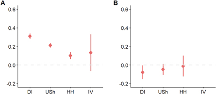
Figure A2. Marginal effects (elasticities) of farm size on the mean and the risk of consumption. Outcomes are (A) log household consumption of food and beverages over the last week, and (B) log variance of log household consumption of food and beverages over the last week. The variance of the IV specification also contains the errors from the first stage regression of farm size on inherited land and cannot be interpreted in the same way. The results are omitted from the figure. Model specifications are DI: OLS with farm size in hectares and district fixed effects, USh: OLS with farm size in monetary value (USh) and district fixed effects, HH: OLS with crop land in hectares and household fixed effects and IV: instrumental variable regression with crop land in hectares, household fixed effects and inherited land as instrument for crop land. All regression specifications include region specific season and year fixed effects (dummies). Standard errors are heteroskedasticity robust and clustered at the district level.
Download figure:
Standard image High-resolution imageThe same increase in farm size reduces the variance of consumption by 0.7% in the specification with district fixed effects and by 0% in the specification with household fixed effects (figure A2, panel B, specifications DI and HH). In comparison, a 10% increase of farm size reduces the variance of income by 1.2% in the specification with district fixed effects and by 0.7% in the specification with household fixed effects (main article, figure 3, panel D). We therefore suggest that farm size has a very similar impact on farm income and farm consumption.
Appendix. C.3. Farm size including forests and pasture
In this section we show our results for our alternative farm size measure including forests, natural vegetation and pastures. All regression specifications are otherwise as in our main specification. Figure A3 shows that the effects are very similar to the estimates of our main specification.
Figure A3. Marginal effects (elasticities) of farm size on the mean and the risk of production measured in revenues (blue) and calories (grey). Outcomes are (A) log production per hectare, (B) log production per unit of labor, (C) variance of log production per hectare and (D) variance of log production per unit of labor. The variance of the IV specification also contains the errors from the first stage regression of farm size on inherited land and cannot be interpreted in the same way. The results are omitted from the figure. Model specifications are DI: OLS with farm size in hectares and district fixed effects, USh: OLS with farm size in monetary value (USh) and district fixed effects, HH: OLS with crop land in hectares and household fixed effects and IV: instrumental variable regression with crop land in hectares, household fixed effects and inherited land as instrument for crop land. All regression specifications include region specific season and year fixed effects (dummies). Standard errors are heteroskedasticity robust and clustered at the district level.
Download figure:
Standard image High-resolution image
Appendix. C.4. Aggregate production with district fixed effects
The following tables present the results on the impact of farm size on aggregate production from tables A4 and A5 but including district fixed effects. In tables A4 and A5 we use two step procedure described in the main text of the article. In tables A6 and A7 we present the same results on the impact of farm size on aggregate production but using multiplicative heteroskedastic linear regression framework based on maximum likelihood estimation (Harvey 1976).
Table A4. Impact of the number of farms and on district level crop production using (OLS estimates).
| R1 | C1 | R2 | C2 | |
|---|---|---|---|---|
| Log farmland | −0.24** | −0.15 | −0.80*** | −0.79*** |
| (0.11) | (0.14) | (0.08) | (0.08) | |
| Log farm number | 0.63*** | 0.47*** | 1.25*** | 1.17*** |
| (0.14) | (0.15) | (0.14) | (0.15) | |
| Observations | 712 | 712 | 712 | 712 |
| R2 (full model) | 0.68 | 0.98 | 0.73 | 0.98 |
Notes. The dependent variable is log output per unit of land at the district level measured in revenues (R1 and R2) and calories (C1 and C2). The independent variables are log total land and log farm numbers. All specifications include district fixed effects as well as region fixed effects and region specific year and region specific season fixed effects (dummies). Specifications R1 and C1 measure farm size in land area while specifications R2 and C2 measure land in land value. Standard errors are heteroskedasticity robust. Significance levels are ***p < 0.01, **p < 0.05, *p < 0.1.
Table A5. Impact of farm size on the variance of district level crop production (OLS estimates).
| R1 | C1 | R2 | C2 | |
|---|---|---|---|---|
| Farmland | −0.20 | 0.17 | −0.28 | −0.04 |
| (0.32) | (0.34) | (0.17) | (0.19) | |
| Farm number | −0.19 | −0.58 | 0.13 | −0.32 |
| (0.39) | (0.42) | (0.26) | (0.28) | |
| Num. obs. | 712 | 712 | 712 | 712 |
| R2 (full model) | 0.45 | 0.46 | 0.45 | 0.41 |
Notes. The dependent variable is the log variance of log output per unit of land at the district level measured in revenues (R1 and R2) and calories (C1 and C2). The independent variables are log total land and log farm numbers. All specifications include district fixed effects as well as region fixed effects and region specific year and region specific season fixed effects (dummies). Specifications R1 and C1 measure farm size in land area while specifications R2 and C2 measure land in land value. Standard errors are heteroskedasticity robust. Significance levels are ***p < 0.01, **p < 0.05, *p < 0.1.
Table A6. Impact of the number of farms and on district level crop production (Maximum Likelihood estimates).
| R1 | C1 | R2 | C2 | |
|---|---|---|---|---|
| Log farmland | −0.31*** | − 0.27*** | − 0.71*** | − 0.68*** |
| (0.07) | (0.07) | (0.04) | (0.04) | |
| Log farm number | 0.48*** | 0.45*** | 0.95*** | 0.92*** |
| (0.09) | (0.10) | (0.06) | (0.06) | |
| Observations | 712 | 712 | 712 | 712 |
Notes. The dependent variable is log output per unit of land at the district level measured in revenues (R1 and R2) and calories (C1 and C2). The independent variables are log total land and log farm numbers. All specifications include district fixed effects as well as region, year and season fixed effects (dummies). Specifications R1 and C1 measure farm size in land area while specifications R2 and C2 measure land in land value. Significance levels are ***p < 0.01, **p < 0.05, *p < 0.1.
Table A7. Impact of farm size on the variance of district level crop production (maximum likelihood estimates).
| R1 | C1 | R2 | C2 | |
|---|---|---|---|---|
| Log farmland | 0.20 | 0.22 | −0.05 | −0.03 |
| (0.13) | (0.14) | (0.07) | (0.07) | |
| Log farm number | −0.54*** | −0.58*** | −0.28*** | −0.35*** |
| (0.17) | (0.18) | (0.11) | (0.11) | |
| Num. obs. | 712 | 712 | 712 | 712 |
Notes. The dependent variable is log variance of log output per unit of land at the district level measured in revenues (R1 and R2) and calories (C1 and C2). The independent variables are total land and farm numbers. All specifications include district fixed effects as well as region, year and season fixed effects (dummies). Specifications R1 and C1 measure farm size in land area while specifications R2 and C2 measure land in land value. Significance levels are ***p < 0.01, **p < 0.05, *p < 0.1.
Footnotes
- 3
See also Western and Bloome (2009) for the impact of logs on the skewness of the distribution.